Blue-Sky Thinking – The design and testing of an Arduino-based UAV

The Challenge

CAD Cutaway
A cutaway CAD render of the aircraft showing the internal wing structure and layout of the electronics.

As part of our second year Aeronautics course at Southampton Uni, we have to undertake a group project. One of the options is to design and build a semi-autonomous UAV flight computer and the wings and circuitry to go along with it. The task requires groups of five to come up with a working design, present it at a series of reviews, build the systems, and then hand over the aircraft to experienced UAV pilots for flight testing at the end of the semester.

Every aspect of the design and testing has to be considered and executed to a tight schedule and on a shoestring budget, then written up into a report after flight testing. Cutting edge programming, design, and manufacturing tools are used to produce very advanced and capable aircraft. I was part of a group which revolutionised the approach to wing manufacture. The whole task encouraged new approaches to problems and encouraged novel solutions to existing problems, which made it very interesting to work on.

This article documents the design, manufacture, and testing process that our group followed, showing some of the elements we built into the design and demonstrating how the resulting aircraft worked.

Design

The starting point of the project is to come up with a detailed list of design targets and concepts to be taken forward into the design phase. This is conducted under significant time pressure, and forces a huge amount of information to be collected and considered before the design can be started.

Concept Sketch of Wing Profile
Initial sketches of the wing profile and internal layout. The flap actuation mehcanism and positioning of spars is considered.

The design phase then builds on concepts and ideas, and develops them further. At this stage, CAD designs begin to be produced, and the subtler corners of the challenge need to be considered. One of the key concerns is fitting all of the scripts and sensor libraries onto an Arduino, which forces an early decision to either scrap some of the sensors, run an Arduino Mega, or use Unos in parallel. This drives the layout, weight, and lift requirements of the aircraft, and subsequently the wing design. We chose to use an Arduino Mega, which gave us more capability and flexibility, but presented more challenge in the fuselage layout and electronics design.

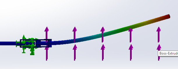
Advanced MatLab scripts and FEA were used to determine the wing profile and shape. Thin aerofoil theory and finite wing theory were captured in scripts and used to optimise the final profile. Stability and handling were evaluated in XFLR, an aircraft modelling program, to evaluate the wing placement, sweep, and taper. Control surfaces were sized according to MatLab simulations and were designed to control the aircraft in gusts of up to 10 kts.

Wing deflection analysis
MatLab-generated graph of wing deflection along the span, subject to an applied aerodynamic load

The structural wing design is a careful compromise between weight, strength, and aerodynamic efficiency. Different approaches lead to wildly varying wing designs – no two wings are the same. Our analysis of the wing requirements led us to specify a very strong wing – one which would stand up to turbulence, transport, assembly, and landing loads without any risk of deformation or fracture. The challenge then came in reducing the weight of the wing to an acceptable level for low-speed flight.

Here we implemented one of the unique aspects of the aircraft. The wing was designed as a two-part fibreglass composite shell, with a spar and ribs providing strengthening. A composite wing in this style had never been completed before, but the achievable strength/weight ratio dwarfed any foam or mylar alternatives, providing solid resistance in the case of a hard landing or high-g turn. The manufacturing process was carefully planned and documented, and the assembly process checked with drawings and CAD to ensure that the timed aircraft assembly could be completed as quickly as possible.

Spar FEA
FEA was conducted on the wing structure to evaluate deflection under aerodynamic loads.

Control

XFLR was used to calculate the stability and control matrices of the aircraft across a range of different attitudes and speeds. We built a MatLab flight dynamics model, implementing the 3D equations of motion of the aircraft, to study the response to perturbations, and to tune the Arduino PID control. With no way of testing prior to the first flight, such a model was immensely valuable in determining the optimal PID coefficients and checking the response of the aircraft in different conditions.

The Arduino flight computer was developed with a Kalman filter in mind. However, to reduce the amount of code required, and to limit the amount of testing necessary to get the filter tuned, a complementary filter was used instead. This combines data from accelerometers and gyroscopes to calculate the angular and linear position and rate of the aircraft. By combining the sensor data, the output is smoothed so that noise has less effect on the results, and avoids challenges such as gyroscopic drift.

The PID control uses a matrix of coefficients, defining the position of every control surface based on the derivative, proportional, and integral terms of the state error. State error is found by calculating the difference between the actual state – the output of the complementary filter – and the target state, which is defined pre-flight to be a straight and level flight state. The PID was tuned using the aircraft model.

Electronics Layout
The (busy) layout of electronics installed in the fuselage

In order to fit everything efficiently onto the Arduino Mega, significant changes were made to the sensor libraries. This reduced the amount of space they took up by nearly 1 kB, leaving this space available for data logging. The space that was saved was used to store a history of the aircraft response to control inputs. While the shakedown flight was taking place, the aircraft was under pilot control, and we used this historical data to fine-tune the PID coefficients. The PID coefficients are functions of the control derivatives, so by determining these more accurately in-flight the PID could be tweaked so that it was closer to the model we had intended. The aircraft had a very basic artificial intelligence system on-board – it would ‘learn’ how it responds to control inputs, and adjust its behaviour accordingly.

Manufacture

The most challenging aspect of the manufacturing was the composite wing. The process was carefully planned: foam moulds were cut, prepared with a release agent (black sacks work surprisingly well) and the fibreglass was cut to the right size. When everything was cut and laid in place, the resin was mixed and applied into the glass fibres. The resin was pressed through the two plies of fibreglass and spread throughout the matrix.

Fibreglass Layup
Laying up the fibreglass in the moulds, using black sacks as a ‘release agent’

The wings were made in two parts – the upper and lower surfaces were made separately so that the moulds could be separated afterwards. The four resulting surfaces were nearly flat, which made it very easy to apply pressure throughout the moulds and force the resin through the matrix as it cured.

The fibreglass was released from the moulds after curing, and was then bonded to a range of carefully designed and laser-cut ribs. The ribs held the surface of the wing in the right shape, adding a small amount of torsional stiffness and providing mounting points for all of the hinges and servos mounted inside. A carbon fibre spar fitted through the ribs, and significant effort went in to getting a perfect press-fit to allow the wing to remain rigid in flight, but be easy to assemble and disassemble on the flight day.

Flap control system
Flap control system, consisting of a servo, a 3D printed control horn, and a bent paperclip.

The wing attachment mechanism was carefully designed, including unique 3D printed spacers and threaded rods to hold the wing onto the fuselage. The mechanism was very light, saving over 100 g against some of the more complex 3D printed clamps used by other groups. The electronics were very carefully planned and put together with a modular design providing flexibility and good assembly speed.
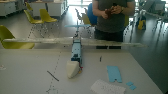


CG check
The completed aircraft undergoing a CG check on the edge of a table, ensuring that it will be stable in flight.

Flight Testing

On the day of the flight test, the aircraft was assembled and prepared for flight. The conditions were not ideal – winds were strong and gusting. They peaked around lunch, just as we were lining up for launch. The first few seconds of flight were smooth and well controlled, and the aircraft responded well to the pilot’s inputs. However, a 13kt gust after a few seconds forced it into a sideslip, and the small tail on the provided fuselage was not enough to correct the slip before the plane hit the ground.

Crash Damage
The aircraft didn’t stand up too well to hitting the ground wingtip first. Note the wing is still perfectly intact, while the fuselage has disintegrated.

Later analysis showed that the aircraft performed as expected given the conditions – it simply wasn’t specified to deal with the conditions it faced. The altitude loss given the gust was not excessive, but since it occurred immediately after take-off there was not enough height to regain control.

The crash showed the robustness of the wing – the fibreglass structure was not damaged at all in the crash and could have flown again… If the fuselage hadn’t snapped and the internal electronics disintegrated as it hit the ground.

Evaluation

A number of new and novel concepts were developed for the aircraft, and it broke new ground in a number of fields (double entendre very much intended). All of the design work and validation came together to produce an aircraft which behaved as expected – unfortunately in conditions it wasn’t designed for.

The project as a whole required a very interesting approach to project management – the electronics, wing, and controls were largely independent in their operation on-board the aircraft. The coupling occurred in the design phase, where the sizing of components and the layout of electronics affected the wing design. The wing layout and modelling also influenced the control systems.

The modelling that was done to ensure that the aircraft performed properly, and to tune the control systems, was very advanced and proved to be a reasonable challenge. It required a different approach to many time-dependent models due to the impact of the controls. The post-flight analysis and correlation checks between flight data and models showed the difficulty of dealing with sensor noise and environmental impacts on the aircraft.

The challenge itself also showed that getting an aircraft to fly is not a huge challenge – anything with a decent wing and a centre of gravity in the right place will fly. However, building something robust, reliable, and efficient is a much bigger task. There is a big difference between a working aircraft and an optimal aircraft, and the latter requires careful specification because it can easily be taken out of its comfort zone.

The bottom line is that this design and manufacture task has allowed a showcase for a huge number of different skills and tools. Designing a UAV is relatively easy, designing an autonomous UAV is hard, and designing a robust, efficient UAV is a significant challenge.

Blue-Sky Thinking – The design and testing of an Arduino-based UAV

Active Suspension: Kinematics and Control Part 2

The previous article in this series detailed the principles behind our suspension modelling and the way in which we will go about designing the system. The development of the system is intended to be a two-year project, with much of the preliminary work done this year before a system is designed from the outset for competition in 2017.

Over the last few months, in parallel with the design of a passive system for 2016 competition, we have built up the model. This has helped us to validate the design and validate the model simultaneously; this year’s geometry is a comprehensive set of coordinates that can be used for testing.

The development of the model has presented some interesting challenges, and one in particular is how to actually define the motion of the suspension. There are many linkages which all need to move synchronously and as a result the motion is nonlinear, with components of rotation, translation, and occasionally twist in the parts.

We also have a very cool way of integrating the system with our CAD work to streamline the design process.

We can see an output of how the system looks as it moves.

Dynamic Suspension Model

The custom dynamic model has been developed and refined to represent the movement of the suspension. Understanding the way that the suspension linkages move in tandem is key to controlling this movement. In particular, the motion of the push/pull rod in response to vertical suspension travel needs to be known.

The sensors for the suspension will be mounted on the pull rod or rocker. If we are to properly control the vertical position of the wheel, we need to know how the vertical position is related to the push/pull rod travel. We also need to know how to work the system in reverse, so that the actuator can be positioned or forced as required.

The dynamic model is the first step towards a full implementation of a kinematic model, which we can use to specify the forces required in the actuator. There are two main ways in which a system can be developed, and each has its own benefits. We are using a bespoke model programmed in C#, which will allow event based and functional programming as required.

Vector Model

The first option for implementing a model to investigate how the suspension travels is to define the position of a single point, and solve all of the contact constraints in the system as this point moves. Since we are interested in the motion as the suspension travels up and down, it makes sense to move the contact patch in the first instance.

All of the points in the car are defined using XYZ coordinates, which means it is trivial to generate and manipulate vectors in the suspension. If the vectors defining all of the points are used correctly, it is possible to calculate centres of rotation and motion paths.

The contact patch is rigidly fixed to the upright, so the motion conducted by the contact patch will match the motion of the upright. The most common way of implementing this motion constraint is to rotate all parts by a very small angle around the same axis. It can be shown that this maintains the shape and internal dimensions of the system.

The axis of rotation is determined as the axis normal to the forced direction of motion of two components. For a double wishbone setup, the axis of rotation is equivalent to the instant centre of rotation in the system.

Once the upright has been moved in this way, we need to find the new position of the steering, pull rod, rocker, and spring. These are all implemented in a similar way. The constraints are the fixed link lengths of the steering arm and pull rod, and their corresponding fixed ends. Once the position of the upright axis is defined, the steering arm upright end can only move on a circular path around the upright. It can also only move on a sphere, centred at the end of the steering rack.

Resolving these two constraints gives only two points in space that the upright pickup can be located. We find the location of the point which is closest to its previous location, representing a smooth motion, and then rotate the upright around its axis until the steering pickup point meets the required location.

Code used to find the location of the steering pickup on the upright. It finds the intersection of a sphere and a circle.

The pull rod is similar – the rocker pickup point can only move on a sphere centred at its pickup point on the lower wishbone, and a circle around the centre of the rocker mounting on the chassis. Between these two points, we can find the location that it must have moved to, and rotate the rocker until the points match. Once rocker rotation is known, the spring length can be calculated, and the position of any active actuator can be determined.

Once all of these relations are defined, it is comparatively easy to run a sweep from the contact patch end and find the positions of the actuator, but just as easy to run the sweep in reverse, as we require.

If the system is event based, so that any change to a coordinate forces update of all of the other relevant systems, it becomes very easy to implement steering, bumps, and move towards a kinematic model which evaluates suspension travel in response to forces.

Equation Driven Model

The second method is to encode all of the above constraints, on fixed positions and link lengths, into a single function which defines the way that each point responds to motion of another. This equation is re-evaluated for each point every time the system is moved.

The motion of all of the points on the upright is governed by the intersection of their possible motion paths, as before. However, rather than solving all of the constraints as the parts move, and adjusting the positions accordingly, the equations handle the positioning, which makes each individual move more computationally efficient.

It is also trivial to adapt the equations to deal with forces if necessary, because the geometry and travel is already in place. This may simplify later stages of the calculations and programming.

More in-depth studies could be conducted, or more iterations run in each sweep, to reduce the accumulation of positional errors. However, it is not possible to reverse this method as easily as the vector method. It is a trade-off based on what we expect the system to do, and the resources that will be available to complete the tasks.

SUFST Suspension Model

I chose to implement a vector-type method in the SUFST suspension model. This means it can cover all forms of steering sweep, suspension travel, and active suspension modelling if necessary. The kinematic analysis will have to be handled separately and at a later time.

This is not to say that the equation driven model is inherently worse, because it is very effective for certain scenarios. The choice for our model is based on the most effective system for our particular situation and design brief.

The reference points used on the front corner of the suspension wireframe model.

CAD Integration

One of the neatest parts of this model is the integration of the suspension geometry with

our SolidWorks models. In a couple of clicks, we can export the coordinates of the suspension geometry from our CAD wireframe model and import them into the suspension model. We can sample a design iteration in around a minute, allowing us to run through multiple design changes very quickly if necessary. For optimising things like the Ackermann steering, rocker motion ratios, and dynamic camber change – all of which can be assessed through the suspension model – this is a very valuable tool.

It is done through the use of VBA macros in the SolidWorks program, and the location of reference points on the critical suspension nodes in the sketch. The macro scans for a specified reference points in the suspension setup, and measures their location relative to the origin to get the XYZ position. This is written to a csv file, along with an identifier for the point.

The coordinates can be exported on separate lines

Or they can have additional information specified, with the XYZ coordinates tabulated.

The coordinates can be exported on separate lines


The C# program can read these csv files and load the coordinates directly into its model, overwriting any coordinates it had stored but maintaining other system parameters and settings. Since no calculations are performed in the system until we specifically move a part, there is no need to regenerate equations at this point – configurations can be freely swapped to investigate the effects of each.

The macro has been written in such a way that the output of the file can be modified very easily. We can set the coordinates to be output in just about any format, which means they can be imported directly into any program – Adams, other proprietary systems, our own system, Microsoft Excel, etc. – as and when we need them. The use of simple macros in this way has massively streamlined our design process and will prove useful for future years designs too.

Further Development

The next steps will focus on implementing an actuator into the system, and quantifying the relationship between actuator position and wheel travel. This is likely to be non-trivial due to a variable motion ratio as the rocker rotates.

Load transfer through the system will also be investigated to see how the actuators affect load transfer and peak load on components.

We are also in the build phase of the 2016 passive system – parts have been sent to manufacture ready for assembly at the same time as the chassis – and updates on that will follow soon.

Active Suspension: Kinematics and Control Part 2

Two by Two: 2048 AI Chain Building

The AI

The AI I am building for 2048 will be written in C++ and imported into the C# game. It is written in a different language for two primary reasons – firstly because using pointers and references significantly reduces the memory requirements and increases the speed of the program when searching through potentially large grids of cells, and secondly because I would personally like to get better at the language through practice.

The speed advantage is not to be ignored. It is possible that the AI could be adapted later to search at greater depths, in which case the time complexity increases rapidly, along with total time. It is also possible that the AI could be asked to perform on larger grids – the UI has the capability to play on grids up to 100 cells square, and that requires a lot of searching and a lot of memory if references are not employed.

The Principle

The chain starts at 64 and stops at the 8

When playing 2048, one of the most effective strategies is to build chains of ascending power of two. This means that once the chain has been completed down to a 2 or 4, when a new cell is added to the board, it can be joined with the end of the chain to double the final cell. Each subsequent cell in turn can be doubled as it is adjacent to the most recently improved cell, up to improving the largest cell on the board having combined all of the cells in the chain.

However, before the chain can even be created, there are a few ways that the available moves can be narrowed down to make searching more efficient. This includes testing how many moves are possible, and whether the chain can even be built at all: As we will see later, the chain can only be built if there is a cell in the corner of the grid.

Checking the Grid

The first check that is done on the grid is to check which directions are valid moves. It is clearly not worth checking if a move in an impossible direction is best. A side effect of this is that if only one move is possible, it can be selected without doing any further analysis.

The board is dangerous in this situation, because only one move can be made

It is also possible for the board to become ‘dangerous’, if a particular situation arises where the newly spawned cell can leave the board in a situation where there is only one possible move, and it will move all of the cells on the board. This is likely to mess up the grid, and should therefore be avoided – a move which causes a dangerous board is ‘unsafe’. The situation arises when a move would leave all rows and columns either full of cells or completely empty, except for one which can be filled by the new cell. This is checked before doing anything more with the AI, and if it leaves only one safe move on the grid, this is selected.

Finding the Corner

The next key step in the AI is to start to build the chain. The chain starts at a corner of the board, and snakes outwards in ways that allow moves without disturbing earlier cells in the chain. The idea is to build large cells on edges or corners, to maximise the number of ways the board can move without disturbing the chain, and while keeping a large, continuous free area for manipulating the small cells. Leaving gaps in the corners means new cells can appear in them, and they are very difficult to improve with limited routes in to the cell. The small cells are kept in the middle, and large cells kept in the corners, to avoid this gridlock situation.

To build the chain requires a seed – the point where the chain starts. This is always a cell in the corner of the board, for reasons mentioned earlier, so if (always near the start of the game) a corner is unfilled, the AI will try to fill it. It chooses the corner to be filled based on the weighting of the grid – trying to keep large cells in corners. The corner with the greatest number of large cells near it is chosen, on the basis that it is best suited to building a chain. If it is unfilled, the AI will move to fill this corner with the largest possible cell. However, if it is filled, this corner cell is used as the basis of the chain.

The chain will search for the 8 and two as shown, and prioritise the 8

Building the Chain

Now the chain can be built in full. This can be done recursively quite neatly, but it is inherently unstable so this AI favours a loop. The chain spreads out from the corner by searching away from the current cell. The next cell in the chain is found by looking for adjacent cells. The final aim of the chain is to collapse it all into one cell, so it is critical that earlier cells in the chain do not move when combining the later cells: this will break the chain. As a result, the AI only searches in directions opposite to those which will not disturb the chain as built so far.

When a cell is found, the value is analysed. The value found defines what happens to the remainder of the chain. If the value is higher than our current end cell, it cannot be added to the chain because this would form a blockage – it cannot be used to double the current end cell. If a cell is found with the same value as the previous cell in the chain, we can begin to collapse the chain because the penultimate cell can be doubled immediately. Otherwise, if a lower value is found, it is set as the current end cell, and is added to the chain. The search then continues.

Code for building the chain of cells

A lower value cell can either be exactly half of the previous one, in which case it forms part of a major chain which is ready to be collapsed as soon as the end cell is doubled, or it can be lower than that, in which case it becomes the start of a minor chain. It will take more than one step to get this cell to a value where it can combine with the previous one. This does not change the logic in this AI, but adding a much lower cell to the chain could be given a lower priority than some other moves in other AIs.

Collapsing the Chain

A move within the chain can only be made if the penultimate and final cells are equal. The AI’s chain builder returns a variable specifying whether this is the case. Once it is established that the chain can accept a move, the direction in which the move needs to take place is found. The two end cells in the chain are retrieved and the row and column indices checked, which establishes the direction in which a move must be made in order to combine the two.

Code for finding the direction of a move, given the two cells that should be combined

It is a result of the careful elimination of different directions in the chain building algorithm that this direction will never be an unsafe direction, so the move can go ahead whenever it is found. If the chain values are halved all the way through, the process will repeat until there is only one cell in the major chain, and then other methods must be used to re-build a chain that can be collapsed once again.

These methods will be described in a later entry.

Two by Two: 2048 AI Chain Building

An AI for 2048

2048Icon
The simple mobile application 2048 went viral around the start of 2014, as a seemingly easy and fast paced online game which was still difficult to complete. As the game became more and more popular, a range of different variations appeared, as did a complementary range of artificial intelligences to solve the variations.

As a game based purely on logic, and with just four possible moves, the game is very well suited to an AI, and I couldn’t resist the challenge of building my own AI.

About the game

The grid before a move...
The grid before a move…
...And after a move upwards
…And after a move upwards


The game is played on a 4 by 4 square grid. Cells are filled with numbers in ascending powers of 2, formed by combining other equal cells on the grid. The four available moves correspond to the four directions, left, up, right, and down, with each move causing all cells to move as far as they can in that direction, while maintaining the original order. If two adjacent cells have the same value, they will combine in the course of the move to form a single cell with double the value, but this cell cannot merge in the same move. Once all moving is complete, a new number is added to the grid in a previously empty cell. This is a 2 90% of the time; the remainder it is a 4.

One example of the board on startup.

To start with, the grid has two random cells placed on it. After the first move, a third cell is added, and the game proceeds as normal. The game ends when no more moves can be made. Each game is different, because the new numbers are added in random locations and have a random value.

Principles of an AI

The reason 2048 lends itself to an artificial intelligence is that there are only four possible outputs (moves). This allows all four of the outputs to be tested easily and quickly to determine the best output. Most systems are based on an analysis of the current game status, testing of all possible future moves, and then re-evaluation of the game situation. The move which adds the most value to the game is then chosen. This can be repeated to a search depth to identify the best move several moves into the future.

However, 2048 introduces a large amount of randomness, which makes searching to any depth inefficient. It would be possible to eliminate some of these eventualities, but a neater solution is to analyse the grid as it stands, and take a deterministic view to the best move. Often, this is easily found, so the deterministic AI has performance advantages. It also acts in a more human way, which tends more to the intelligence aspect of an AI.

I also wanted to avoid, as far as possible, scoring the board against certain measures and adjusting the weighting of these measures. This feels like a sub-optimal process, which leads to a rule-based AI. This means that a list of true-false cases describing board parameters are tested, and whenever a true case is found, a move is generated based on this case.

The AI will be a set of if-else statements, with each if case testing if a move can be found in a certain way. These categories are, for example, trying to fill a corner, or moving to avoid a dangerous situation where the board could be blocked by the next move. There will be more on the AI in later posts.

Building the game

In order to build the 2048 AI, the game needs to be built first. The game and AI are built in C#, so the application uses the WPF framework. This also provides animations and XAML, making the design of the game easy.

Designing the interface using WPF

The board consists of a 4×4 integer array, with blank cells represented by zeros. To move the cells requires a carefully designed algorithm but can be done in O(n2) time, by scanning in the opposite direction to the move. As the grid is scanned, the system keeps a record of the position that the next cell is moved to, and the value of the previous numerical cell. If a cell with the same value is found, it can be merged. Otherwise, any cell is moved to the next free cell. The algorithm is carefully designed to cope with all possible eventualities.

When a move is made, instead of updating the grid through bindings which limits the potential to use animations, the moves made are passed to the UI, which rearranges labels on a canvas. Working this way allows the move, merge, and appear animations to be synchronised. It also means that the game logic is independent of the UI, so the graphics can be changed at any time without affecting the rest of the game.

AnimationCodeThe animations take significantly longer than processing the moves, which means that separating the two leads to lag in the game if moves are not queued. Thankfully, wpf runs the animations in a separate thread, which means with a careful bit of planning the moves can be queued and the board updated in the background, with the animations running on the user interface.

To integrate the artificial intelligence, the AI subscribes to an event on the game, which is fired whenever the grid is updated and ready to receive another move. At this point, the AI calculates the best move, and returns it to the game. This generates a loop, which repeats until the AI cannot find a move.

There will be more in further posts about the development of the artificial intelligence. Now that the framework has been established, development can proceed quickly.

An AI for 2048